


If you have worked with Blender and Cycles for some time, you probably have a good understanding of a few render settings. But I would bet that there are at least a handful of settings you don't know much about. The goal for this article is to explain and explore most of the Cycles render settings and build a better foundation for artists so that they know what happens the next time they press render.
Cycles render settings are found primarily in the properties panel if you click the render tab. That is the camera icon, second from the top. Here we find settings divided into several categories.
This is not a complete beginners guide to Cycles, instead we look at specific settings and discuss what they do.
If you are looking for a beginner's guide, I would encourage you to start in the Blender manual and then check out my article on the light path node.
External content: Blender manual, Cycles
Understanding the light path node is an effective way to see how Cycles handles light and calculates the final color for each pixel in a scene.
Related content: How the light path node works in Blender
Another great resource is this YouTube video from the Blender conference 2019. The talk is by Lukas Stockner.
External content: Blender conference talk - Introduction to Cycles Internals - Lukas Stockner
For learning about shading in Cycles and Eevee, you can start with this guide.
Related content: The complete beginners guide to Blender nodes, Eevee, Cycles and PBR
At the very top we find a few general settings that doesn't belong to any category. Here we can specify the render engine. By default, we can choose between three engines.
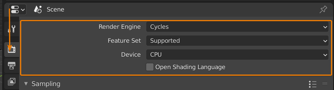
If we have other render engines installed and activated, we can choose them from this list. In this case are looking specifically at Cycles. The primary ray-traced render engine for Blender.
Next, we have feature set. In Cycles we can use Supported and Experimental. If we switch to experimental, we get some additional features we can use. The most noteworthy experimental feature is adaptive subdivision for the Subdivision surface modifier.
This is an advanced feature that allow subdivided objects to subdivide according to how close the geometry is to the camera. The idea is that we can improve performance by adding more geometry closer to the camera where it is mostly visible and save on geometry further away from the camera so that we may save performance.
By the way, if you enjoy this article, I suggest that you look at my E-Book. It has helped many people learn Blender faster and deepen their knowledge in this fantastic software.
Suggested content: Artisticrender's E-Book
If we enable experimental feature set, a new section appears in our render settings called subdivision. If we also go to the modifier stack and add a subdivision surface modifier you will see that the interface has changed, and we can enable adaptive subdivision.
But let's not get too far outside the scope of this article already.
Just below the feature set we have the device. Here we can choose between GPU and CPU. This setting depends on your hardware. If you have a supported GPU you most likely want to use it for rendering. In most cases it improves performance.
Before we can use GPU however we need to go into our preferences and set our compute device. Here we will also see if Blender recognize any supported GPU in your system.
Go to Edit->Preferences and find the System. At the top you will find the Cycles render devices section. If you have a supported Nvidia GPU you can use Cuda.
Since Blender version 2.90, Optix should work with NVidias older series of Graphics cards, all the way back to the 700 series according to the release notes. It is the faster option but lacks some features.
External content: Blender 2.90 release notes
According to the manual these features are supported by Cuda but not Optix.
Also, these are features that are not supported on GPU, instead you must use CPU to enable these.
External content: Blender manual, GPU rendering supported features
If you are a general artist, the features you mostly would need are Baking, the Ambient Occlusion and Bevel nodes. But you can switch between Cuda and Optix at any time.
For AMD graphics cards, use OpenCL. The downside of OpenCL is that we must compile the kernel each time we open a new blend file. Don't ask me what it actually does, but what it means for the user is that we may have to wait, sometimes for several minutes, before we can start to render. Your CPU does this calculation, so it depends on both the complexity of the scene and the speed of your CPU.
If you have an integrated graphics card it most likely isn't supported and you will have to render with CPU. In most systems, this is the slowest compute device for rendering.
You can find the latest data from Blender's open data project where data from the communitys benchmarks are gathered.
External content: Blender Open data
Enough about devices, but if you have CPU enabled, you have the Open Shading Language option available. You need to check this to enable support for OSL. OSL is a scripting language that we can use to write our own code to program shaders. If you are interested in that you can start to read more in the manual here:
External content: Blender manual, Open shading language
As a side note before we leave the general settings, I also want to add that in version 2.91 there is a search feature added to the properties panel so that we can filter settings by searching them by name. If you are reading this in the future, this feature most likely still remain.
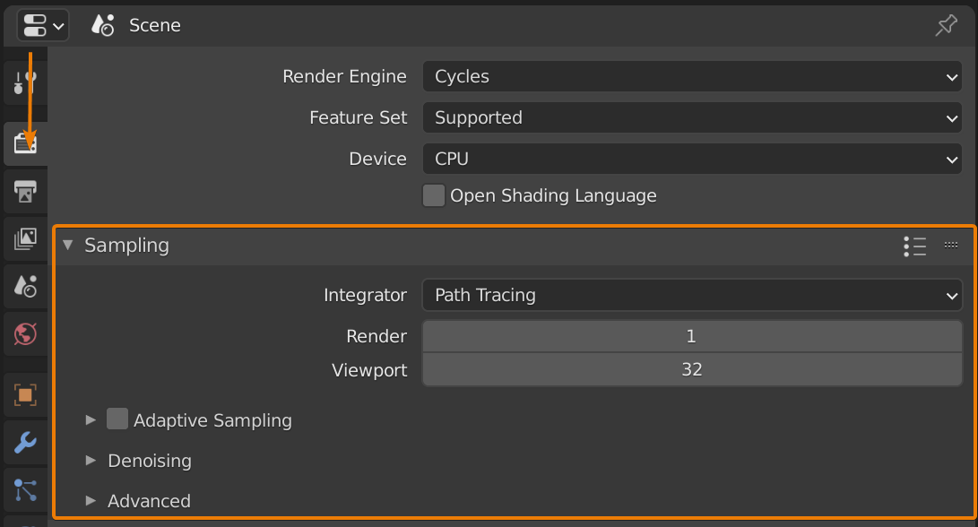
We will start by discussing samples, then jump back up to the integrator.
Samples is a number for how many light rays we let Cycles shoot from the camera into the scene to eventually hit a light, the background or be terminated because the ray run out of allowed bounces.
The goal with shooting light samples into the scene is to gather information about everything in the scene so that we can determine the correct color for each pixel in the final image.
It does this by bouncing around according to the surfaces that is hit and what material properties are detected at each location.
We have several options to control the samples, both in this section and the next, light path section.
If you are looking for a hands-on way of learning how this works in practice, I encourage you to check out the article on the light path node. You can find it here:
Related content: How the light path node works in Blender
The samples are the most well-known setting in Cycles. They are labeled render and viewport. The render count is used for the final renders and the viewport samples are used in rendered viewport shading mode.
You can read up on all viewport shader options and what they do in my guide here:
Related content: Blender viewport shading guide
So, what determines how many samples we should use? It comes down to one thing. Noise.
If your image has more noise than you can tolerate or to be accurate and noise free, we may need more samples. But there are a whole lot of other tools and settings that we should consider tweaking before we increase the sample count to insane amounts. Some of them, we explore in this article.
But as a rule, if your scene is setup correctly, it is my opinion that you should not need to go above 1000 samples. But there are artists that think even one thousand is a way too high number.
At the lower end, I rarely use less than 200 samples. But then again, I don't render many animations. When that occurs, I may make an exception to that rule.
For the viewport sample, we can set this to zero for continuous rendering. For the final render this works slightly different. To render the final render continuously we go to the performance section, find the tiles subsection and here we have Progressive refine. This will change the regular tile rendering into rendering the entire scene at once with infinite samples, allowing the user to cancel the render when it is noise free.
By default, we use the path tracing integrator. While still complex, this is the more basic integrator that gives us equal light bounces no matter what property the surfaces we hit has. It shoots of rays equally making each individual ray faster, but for surface attributes that need more samples to clean up properly and remove noise, it may take longer than the alternative witch is branched path tracing.
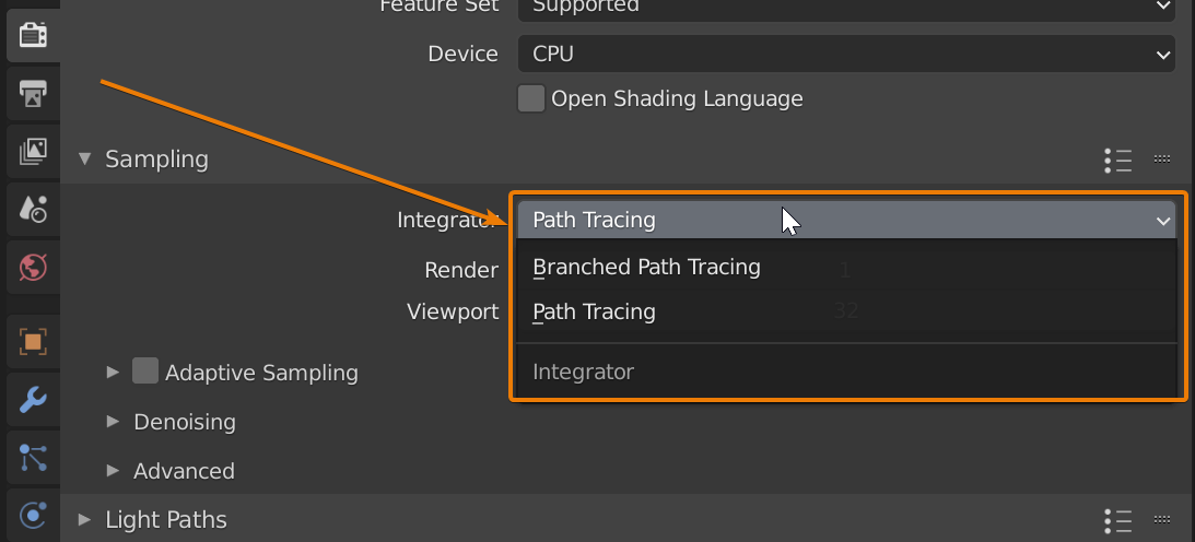
Branched path tracing on the other hand shoot the rays into the scene but at the first material hit, it will split the ray and use different amounts of rays depending on the surface attributes and light.
We can set how many rays Cycles use for each first hit material or feature if we go to the sub samples subsection.

Here we will find a lengthy list of distinctive features that we can define sample count for after that initial ray hit. The numbers here are multipliers.
So, for a diffuse sub sample count of two it will take the render samples and multiply by two and use this number of samples for diffuse material components.
Let's say that we have trouble making our glossy noise-free, we could use branched path tracing to give glossy way more samples so that it can clear up, while not wasting calculations on an already clean diffuse path.
In all honestly, I rarely use branched path tracing. Since it isn't supported by Optix. So instead, I often just crank up the samples. But in those cases when you are sitting with an animation that won't clear up properly, branch path tracing can be an option.
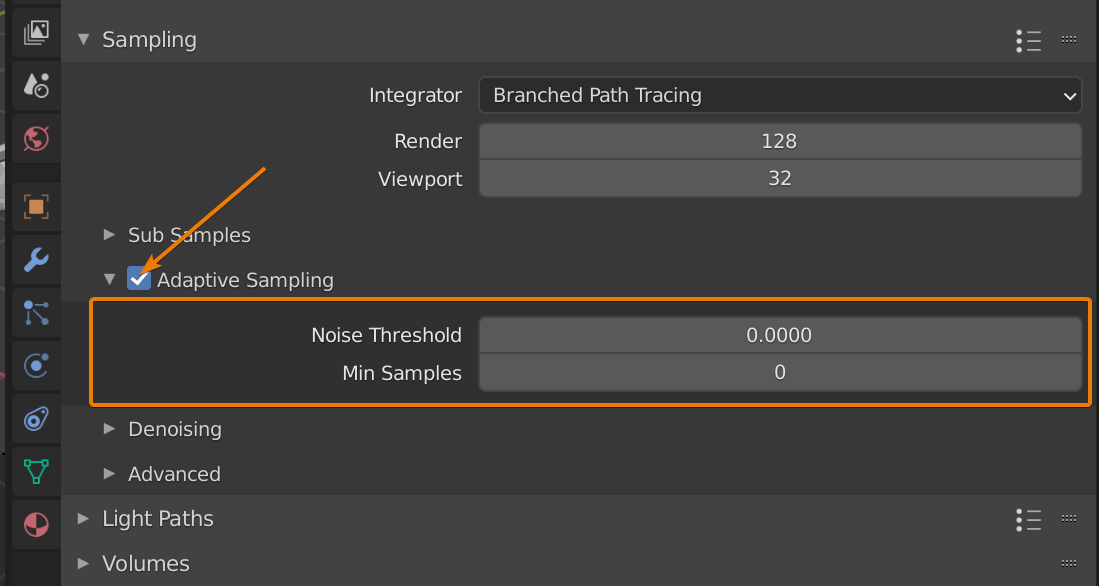
Adaptive sampling appeared in version 2.83. The idea is that Blender will sense when the noise is reduced enough and therefore stop rendering the area while continue render areas that require more samples to become noise free.
According to the 2.83 release notes render times are reduced by 10-30 percent when using adaptive sampling. In my own experience I find the same thing. Generally, render times is slightly faster and I haven't had a render that I could tell much difference from not using adaptive sampling.
We can set a minimum number of samples with the min samples setting, not allowing Cycles to use fewer samples than specified here.
The noise threshold is automatic when set to zero. The lower the number, the longer Cycles will keep rendering until it reaches the samples count or until the noise level has reached the threshold.
In the denoising subsection we can set a denoiser for the final renderer and for the viewport. Since the viewport is denoising in real-time for every sample, we can set a start sample so that the denoiser doesn't kick in before a set number of samples has already been calculated.

For the viewport, we have three options.
Automatic isn't really an option. It will just use Optix if available, otherwise fall back on OpenImageDenoise. Because Optix is the faster option it has higher priority, but it requires a compatible NVidia GPU.
For the viewport, it is pretty simple, enable, choose your AI and from what sample to start denoising.
Also, don't forget to check out the E-Book. I am convinced that it will help you learn Blender faster. That is why I made it. Click the link.
Suggested content: Artisticrender's E-Book
For the final render it is still not complex, you can just turn denoising on, choose your denoiser and Blender will spit out a noise free render for you.
For the render denoiser, we also have another alternative called NLM. While the other options are AI based denoisers, NLM is a traditional built-in denoiser that depend on the parameters we feed it. In general, it doesn't give as satisfactory results as Optix or OpenImageDenoise.
Personally, I think that OpenImageDenoise gives the absolute best results.
Anyway, the denoiser we choose for rendering also affect what data the denoising data pass produce. Optix and OpenImageDenoise produce the same passes and as far as I can tell, they look identical.
These are the passes:
On the other hand, NLM produces four additional passes:
We may want to have any of these passes available when we export to another application, but within Blender they are rarely used. With NLM the Denoising Normal, Albedo and Depth often come out grainy or blurry.

The only passes we use consistently are Denoising Normal and Denoising Albedo together with the Noisy Image that gets produced if we use a denoiser at all.
We use these together with the denoising node in the compositor. The denoising node uses the OpenImageDenoiser to denoise in post instead of denoising interactively at render time.
My preferred method of denoising is therefore to use Optix, interactively and enabling the denoising data pass so that I can use OpenImageDenoiser in post with the denoising data passes produced by Optix. This way I can choose what denoiser without having to render twice.
Here is a guide on how to use the OpenImageDenoiser through the compositor.
Related content: How to use Intel denoiser in Blender
Also keep in mind that we need to enable interactive denoising to have access to the denoising settings for any of the denoisers. When interactive denoising is activated in the render settings we find these settings in the view layer tab in the denoising section. Note that we can also turn off denoising for individual render passes here.
Here we begin with a seed value, this is something we see all over Blender. It is a value that changes the pattern of random distribution. In this case, it is the random distribution of the Cycles integrator. This will give us a different noise pattern across the image. The clock icon will change this value between each frame when rendering animation. This can help us turn the left-over noise into a film grain look instead.
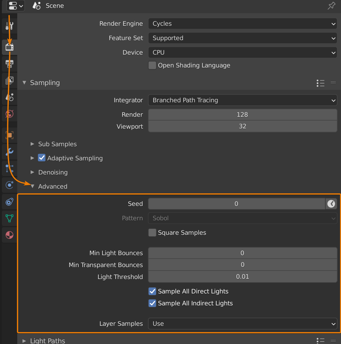
The pattern is the distribution of samples. You want an even, but random distribution and there are two ways to achieve this in Blender. Sobol and multi-jitter. Sobol is the default for now, and the difference between them seem to be un-noticeable in most cases. Sometimes though, one or the other come out on top by a clear margin but to me it has not been obvious why.
While researching this, what I found was that there have been many discussions around this and at times, multi-jitter seem to have had an advantage but for the most part it seems to still be about opinion.
There are two types of multi-jitter and if you turn on adaptive sampling the progressive multi-jitter will be the used pattern and this setting will be grayed out.
The square samples checkbox will take our sample count and multiply it by itself for the final sample count. It is just a different way of calculating samples.
Moving right along, with the min light bounces we can override the lowest allowed bounces for all individual ray types and while this is set to 0 this is disabled.
For instance, if we have diffuse bounces in the light path section discussed below set to 3 and the min light bounces set to 5 here, we will use five bounces.
When the minimum light bounces are met, rays that contribute less will be terminated.
The min light bounces setting can help reduce noise, especially in more complex scenarios with glass, liquids, and glossy surfaces but render times can be affected considerably.
Min transparent bounces can also help reduce noise in scenes that use transparent shaders. Not that this is not, for instance a glass shader that uses transmission.
The light threshold is the minimum amount of light that will be considered light. If the light is below this threshold it will be considered no light. This is so that the render engine don't have to deal with calculations that contribute minimal amount of light and waste render-time.
When we use branched path tracing, we have two additional advanced settings. These are sample all direct light and sample all indirect light.
Just like we can give different material properties or features different amounts of samples with branch path tracing, we can give different lights different amounts of samples when these are turned on.
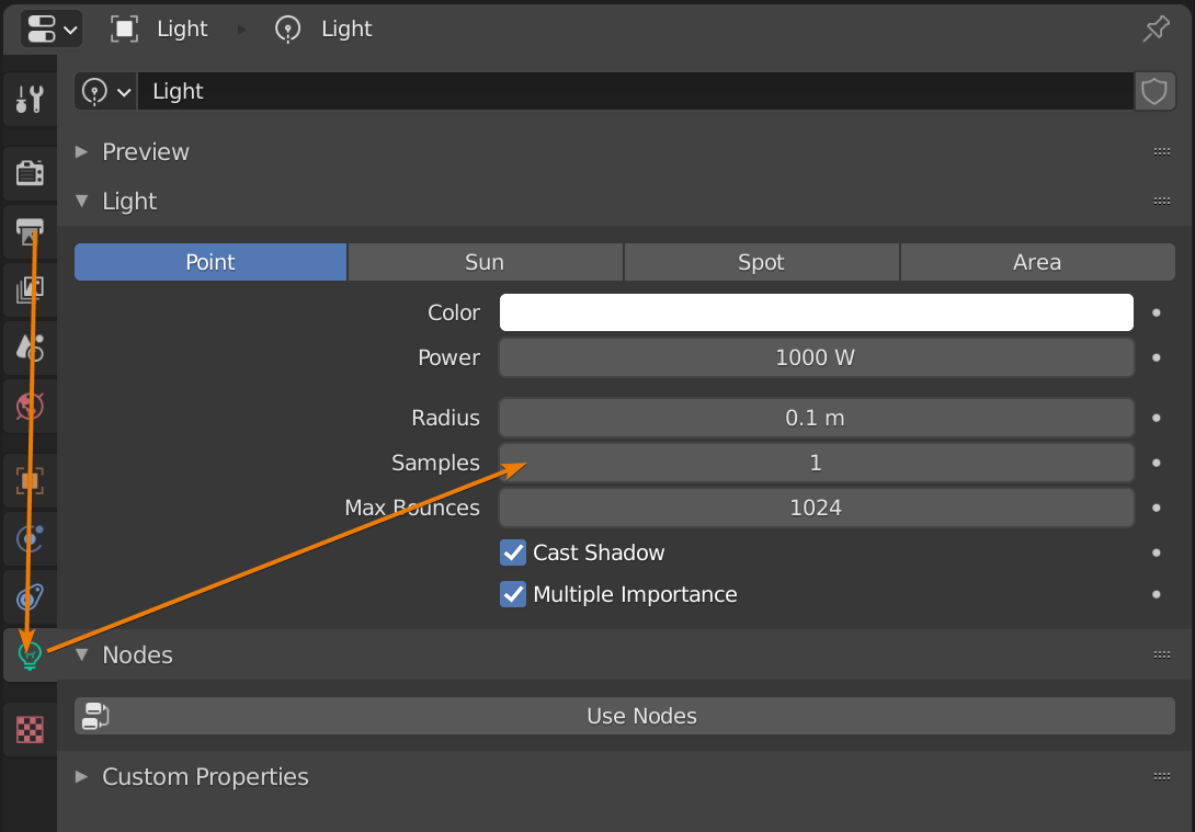
If you select a light and go to the object data properties, you will see that you have a sample count here. This sample count is multiplied with the AA samples for this light when using branched path tracing and these settings are turned on.
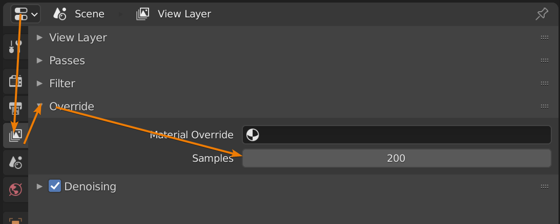
At the very bottom, another setting can appear called layer samples. If we go to the layer tab and open the override section, we can set the number of samples we want to calculate for this view layer separately. If this is set to anything but zero for at least one view layer the layer samples setting becomes visible.
It gives us three options.
Set to use, we will use the override and set the samples to whatever value is in the view layer tab. Ignore will ignore any samples override at the view layer level. If set to bounded, the lowest number of the two will be calculated.
The light bounces are one step closer in on the details compared to samples. Here we decide the maximum number of bounces we want for each of the rays shot into the scene.
If it isn't open, expand the max bounces subsection. We have an overarching value called Total. When this amount of bounces is met by any ray, we terminate it.
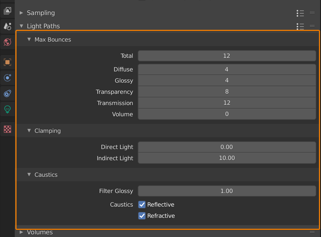
Below the total value are the individual ray types and how many bounces we allow for each. I have found that in many cases these values are set too high and we can save a lot of render time by decreasing these values.
These are the values I generally start with.
This is what fits my work most of the time. You likely need to adjust these settings according to the kind of art you create. Here are a few examples.
For instance, if we use a lot of objects with transparent shaders behind each other. In those cases, a too low transparency bounce value will totally obstruct the view or have the transparency cast a shadow. Often this result in a way darker looking material than we want or black spots where the ray is killed rather than continue through the material.
But transparency is also expensive and adds to render times, so we don't want to increase this higher than we need.
A similar problem may arise with glass shaders. If the transmission setting is too low, we may get black or dark artefacts in the glass. This is more apparent in shaped glass with more curves and details.
In interior scenes lit with light coming through a window, we are often better off with faking it slightly by combining the glass with a transparent shader. Filtering all light from a scene through an object with a pure glass shader often give us more headache than it is worth.
Just an additional note. With the volume bounces at 0 it will still allow a single bounce. When we set this to any higher number, that is equal to the additional bounces, or scatters allowed.
Moving right along to the next subsection. Here we find clamping. We have two clamping settings. Direct light and indirect light.

These values limit the maximum amount of allowed light recorded by a sample. This can help reduce fireflies in a render when there is a probability that a sample goes haywire and records an excessively high number, resulting in a pixel getting rendered white.
Clamping breaks the accuracy of the light though so it should be left as a last resort when we are having trouble with fireflies. A value of 0 will turn off clamping.
Caustics is the play of light that happens when light passes through something like a water glass and throws a light pattern on an adjacent surface.
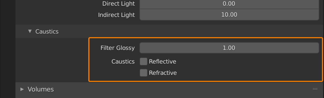
It is often incredibly beautiful and a desirable effect. The problem is that it is incredibly expensive and prone to creating fireflies. It also requires an enormous number of samples to smooth out.
If you require caustics in your scene you are often better of faking it than letting Cycles calculate it for you. So, turning these off is a quick way to ease up the calculations Cycles must make.
The filter glossy setting I find especially useful. This is another setting where we balance accuracy for performance. Filter glossy will give glossy components a blur to reduce noise.
I find that in many cases, just a bit of filter glossy can allow you to get away with fewer glossy bounces and speed up renders with minimal cost to accuracy.
But it depends on how picky you are with accuracy. Personally, I prefer a nice image rather than an accurate one.
In Cycles volume settings, we have a step rate for the viewport and final render as well as a max steps setting.
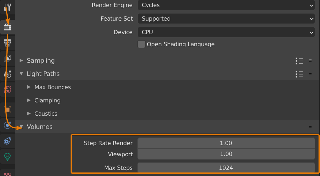
A step, is a point inside the volume that is a potential place where a scatter, absorb or emission might happen depending on the type of shader. The chance that such an event occur at a step is based primarily on the density.
We used to control a value called step size. This was a value set in meters or blender units. This would set the distance in the volume between each potential bounce for a ray.
These days, Blender automatically set the step size and instead we control this step rate value. This is a multiplier of the automatically set step size.
This means that, before, we had to adjust the step size according to the size of the object. Now, the step rate is instead a value that is in relation to the step size so we no longer need to adjust it in relation to the size of the object, but instead, in relation to how frequent we want the bounces to happen inside the volume regardless of its size.
A value of 1 will leave the step size Blender set, a value of 2 will multiply the step size by 2 etc.
The max step is a safety net so that we don't end up in an infinite number of steps. Instead the steps are terminated once this number of steps is reached.
When we create hair in Blender most settings are going to be in the particle system, the particle edit mode and the shader. However, there is one setting that is global for the entire scene. That is the hair shape. We have two options here.
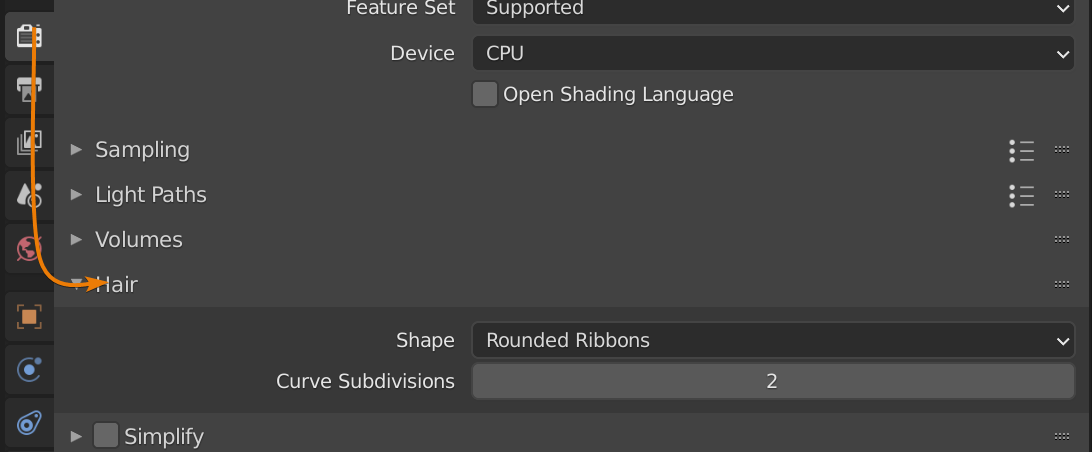
Frists, rounded ribbons that will render as a flat object with smoothed normals so that it doesn't render sharp edges when it curves. This is the faster alternative.
We can set the curve subdivision while using this setting to smooth out the curve along the hair.
But if we zoom in, we will see that the curve is jagged and sometimes we see artefacts as strands beside the hair particle. So, if we need a hair closeup, we are better off with the second option 3D curves.
This is slower to render but holds up better when we zoom in for really close shots of the hair.
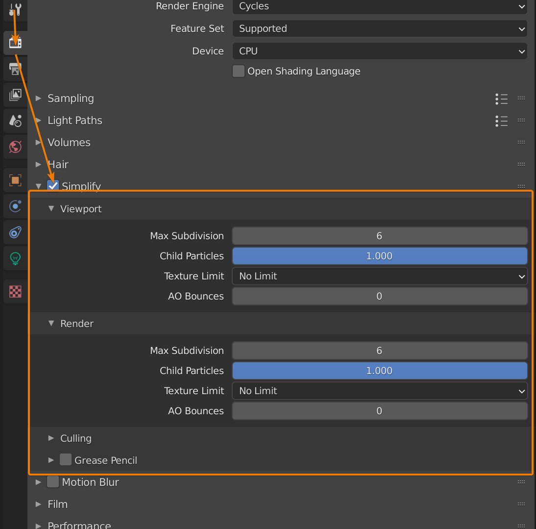
At the simplify settings department we have two copies of the same settings, one for viewport and one for final renders.
After that we have a culling section. If we try to google "culling" to find out what it means we get this answer:
"reduction of a wild animal population by selective slaughter."
Not very helpful for us. Also, I don't really know what to think about the fact that this is part of the Simplify section.
At last we have the grease pencil section that we will skip since it is outside the scope of this article. But let's start at the top.
In the viewport and render sections we have max subdivision. This value will limit any subdivision surface and multiresolution modifier in the scene to this amount of subdivisions.
A great way to limit the amount of geometry in a scene with objects based on any of these modifiers without having to adjust every single object.
Next is child particles, this will multiply the number of child particles with whatever number we set here. So, if we set 0.5 only 50% of the child particles in all our particle systems will be rendered. Note that it only applies to child particles and not the emitted particles.
The texture limit will reduce the size of textures used to any of the limits we choose here. Pretty handy when you are working on a large scene and suddenly realize that you ran out of memory to render it.
The AO bounces is a bit special. It will stop Cycles from using global illumination after the set number of bounces, then AO will be used instead. I explore this more in this article:
Related content: Ambient occlusion in Blender: Everything you need to know
Let's get back to the culling section. It doesn't have anything to do with animals. Instead these settings will help us automatically remove any objects outside the view of the camera as well as at any given distance from the camera.
For an object to take part in culling, we need to enable culling for that specific object. To do this we go to the object properties, find the visibility section and in the culling sub section we can enable camera cull and distance cull.
Here is a little Blender trick for you, to change a setting like this for all selected objects, set the setting you want for the active object, then just right click and select copy to selected.
Also, to use culling on particle systems, we enable culling on the object we distribute and not on the emitter.
Once back in the simplify settings we can enable or disable camera culling and distance culling.
For camera culling, this value decides how far away outside the camera view we cull away objects. You can think of it as the higher the value, the larger the margin before culling begins.
For distance culling, this works the opposite way. The higher the distance, the further away we allow objects to render. Just keep in mind that at a value of 0, distance culling is turned off. This means that as we go from 0 to a low value, such as 0.001 we go from rendering everything to limiting the distance to this ridiculously small number. Essentially making a jump from rendering everything at 0 to rendering almost nothing at 0.001.
Keep in mind that the distance culling does not remove objects far from the camera within the cameras field of view. With both active, distance culling adds objects back in based on the distance.
In the film settings the most used settings is transparent. By checking the transparent subsection the world background will render transparent, but it will still contribute to the lighting.

This is a very useful setting in many cases. For instance we can composite an object over a different background or we can use this to render a decal that we later can use as part of a material.
Another example is to render a treeline or similar assets. I touch on this briefly in the sapling add-on article found here:
Related content: How to create realistic 3D trees with the sapling add-on and Blender
With the transparent subsection enabled we also get the option to also render glass transparent. This allow us to render glass over other surfaces. The roughness threshold will dictate at what roughness level the breakpoint is and we render the original color instead.
Let's head back to the top of this section and cover exposure. The exposure setting decides the brightness of an image. It allows us to either boost or decrease the overall brightness of the scene.
We find this same setting in the color management tab. The difference here is that the exposure from the film section applies to the data of the image while the color management exposure applies to the view.
We won't see the difference in Blender since we work with both the data itself and the view. The difference becomes apparent when we separate the view from the data. We can do this by saving to different file formats.
If we save the render as a file format that is intended as a final product, such as a jpeg, we will get the color management applied and therefore also the color management exposure. But if we export to a file format that is intended for continual work such as OpenEXR we will only export the data and the color management exposure setting won't be part of the export.
The difference is subtle, but important if you intend to do additional processing in another software.
At last we have the pixel filter setting. This has to do with anti-aliasing. The feature that blurs edges and areas with contrast for a more natural result, hiding the jagged edge between pixels.
The default Blackman-Harris algorithm creates a natural anti-aliasing with a balance between detail and softness. Gaussian is a softer alternative while box is disabling the pixel filter.
The pixel filter width decides how wide the effect stretches between contrasting pixels.
The performance section has several subsections, this time, we will start from the top where we find threads.
This section is only applicable to CPU rendering and we can change how many of the available cores and threads we will use for rendering. By default, Blender will auto-detect and use all cores. But we can change this to fixed and set the number of cores to allocate. This is most useful if we intend to use the computer while we are rendering, leaving some computing power left for other tasks.

In the tiles subsection we can set the tile size. We handle an array of pixels to compute for each computational unit. Either for each graphics card or for each CPU core. The tile X and tile Y values will decide how large each chunk should be that is handled at a time by each computational unit. As a tile finished rendering the computational unit will be allocated a new tile of the same size until the whole image is rendered.
Generally, GPUs handle large tiles better while CPUs handle smaller tiles better.
For GPU you can try either 512x512 or 256x256 as starting points and for CPU, 64x64 or even 32x32 are good sizes to start with. Keep in mind that the scene and your specific computational unit may have a very specific ideal tile size, but the general rule is often good enough for most daily use.
Just one thing, if you find this article helpful, perhaps you will find my E-Book helpful as well. It has helped many people become better 3D artists faster.
Suggested content: Artisticrender's E-Book
Let's continue
We can also set the order that tiles get picked. As far as I know there is no performance impact here. Instead it's just a matter of taste.
The last setting in this section is progressive refine. We explained this earlier. But what it does is that it allows us to render the whole image at once instead of a tile at a time.
This way we don't have a predefined number of samples, instead samples are counted until the render is manually cancelled. This is a good option if you want to leave a render overnight.
For animations, this setting will make it so that we render the entire frame at a time, but it won't render each frame until manually cancelled. Instead it will use the sample count as normal.
This is an advanced section that I don't fully understand, but I will do my best to explain what I know. Let's start with Spatial Splits. The information that I found was that it is based on this paper from NVidia.
External Content: Nvidia Spatial split paper
In this paper they prove that spatial split renders faster in all their test cases. But there are two parts to a render, the build phase, and the sampling phase.
In the build phase Blender uses something called BVH (Bounding volume hierarchy) to split up and divide the scene to quickly find each object and see if a ray hit or miss objects during rendering.
Check out this Blender conference talk for a more complete explanation.
External content: Blender conference talk - Introduction to Cycles Internals - Lukas Stockner
My understanding here is that traditional BVH is a more "brute force" way of quickly dividing up a scene that in different cases end up with a lot of overlap that needs to be sorted through during the sampling phase.
Spatial split uses another algorithm that is more computational heavy, making the build phase take longer but, in the end, we have a BVH that overlaps significantly less making the sampling phase of rendering quicker.
When spatial split was first introduced in Blender it did not use multi-threading to calculate the BVH, so it was still slower than the traditional BVH in most cases. However, spatial splits were multi-threaded quite some time ago and shouldn't have this downside anymore.
External source: developer.blender.org
However, it is still a slower build time and my understanding is that the build time is always calculated on the CPU so if you have a fast graphics card and a relatively slower CPU like me, the difference is going to be pretty small since you move workload from the GPU to the CPU in a sense.
My own conclusion is this: Use spatial splits for complex single renders where the sampling part of the render process is long if the performance between CPU and GPU is close enough to each other.
For simpler scenes, there is no need, because the build time will be so short you won't notice the difference. For animations, Blender will rebuild the BVH between each frame, so the build time is as important as the sampling and we have much more wiggle room when it comes to improving the sampling as opposed to the build time.
The next setting is Use hair BVH. My understanding of this is that if you have a lot of hair in your scene, disabling this can reduce the memory usage while rendering at the cost of performance. In other words, use this if your scene has a lot of hair and you can't render it because the scene uses too much memory.
The last setting in this section is BVH time step. This setting was introduced in Blender version 2.78 and it helps improve render speed with scenes that use motion blur. You can find out more in this article.
External content: Investigating Cycles Motion Blur Performance
It is an older article benchmarking version 2.78 that shows how motion blur renders faster on CPU. This may or may not be true any longer since much has happened to Cycles since then.
But in short, the longer motion blur trails and the more complex the scene is the higher BVH time steps. A value of 2 or 3 seems to be good according to the article above.
Here we find two settings, save buffers and persistent images. Information about these are scarce on the Internet and the information you find about them is often old. After some research and testing, this is what I found.
Let's start with Save buffers. When turned on, Blender will save each rendered frame to the temporary directory instead of just keeping them in RAM. It will then read the image back from the temporary location. This is supposed to save memory during rendering if using many passes and view layers.
However, during the limited testing I have done, I haven't found any difference.
You can go to Edit->Preferences and in the file path tab you will find a path labeled temporary files. This is the location these files will go to.
They will end up in a sub-folder called blender followed by a random number. Inside the folder each render is saved as an exr file named after the blend file, scene, and view layer.
These folders do not persist. They are limited to the current session. If Blender closes properly, Blender will delete this folder as part of the cleanup process before shutting down.
Even if these files are loaded back into Blender, we still use the Layer node in the compositor to access them, just like we would without save buffers enabled.
Persistent images will tell Blender to keep loaded textures in RAM after a render has finished. This way, when we re-render, Cycles won't have to load those images again, saving some time during the build process while rendering. The downside is that between renders, Blender will use a whole lot more RAM than it usually does and potentially limiting RAM availability for other tasks between renders. But if you have piles of RAM left over, please use it and save yourself some time.
I have found this to be especially useful when rendering animations as well. If this is disabled, Blender will reload textures between each frame. But enable it and Blender will keep those images loaded between frames.
After an animation has rendered, we can uncheck this and Blender will release the memory instantly.
In this section we find settings that can help us optimize the viewport rendering by limiting the resolution. By changing the pixel size we can make the drawn pixels bigger. At1x we render them at 1x1. At 2x we render them in 2x2 pixel sizes etc.
The automatic option will use the interface scale that we can find if we go to edit->preferences and find the interface section. There we have a resolution scale value that changes the size of the interface.
The start pixels will set the size of pixels at the start, this will be refined to the pixel size setting over time.
The last setting which is denoising start sample will make Blender wait until this many samples has been calculated before denoising kicks in to refine the image.
There is a huge diversity among render settings, and it can be hard to navigate what we actually need at any given time. At the end we just want the right look with the maximum performance possible, mitigating any render errors.
If you came all this way, I hope that you gathered some knowledge and if you ever feel lost while trying to figure out Cycles render settings in Blender, you are not alone. But you are always welcome back to this article for repetition.
Thanks for your time.
