


Geometry nodes has now been around for a while and the time to get into it is now better than ever. In this fundamentals guide we will cover topics such as how to setup geometry nodes, the core fundamental tools we need to understand to be effective with it and touch on what we should and perhaps should not do with it.
Geometry nodes is a node system that allow us to procedurally control the data in a mesh or curve object. We can also animate any value within the node graph and it interact with our object in the form of a modifier in the modifier stack.
Related content: How modifiers work in Blender, an overview
Let's dive in and learn about this new fantastic tool.
Geometry nodes is a system to procedurally build upon different object types in Blender to create various tools, scatter and other procedural effects.
Here is a list of things we could potentially do with geometry nodes.
Related content: How to use a particle system in Blender to scatter objects
This is not an extensive list by any means. Only our imagination sets the boundaries for what we can do with this tool.
However, keep in mind that even if there is a lot we can do with geometry nodes, it does not make other tools in Blender obsolete.
In fact geometry nodes complements a lot of the tools and techniques we already use by enabling us to use procedural functions to enhance these other features. For instance, we can use geometry nodes to tell what parts of a mesh should have what material or scatter objects with much more control than we previously could with a particle system.
Before you get started with geometry nodes I recommend that you have some experience with shader nodes. You can read a beginners guide here:
Related content: The complete beginners guide to Blender nodes, Eevee, Cycles and PBR
We will start from the beginning but rapidly increase the difficulty and add concepts through the article. So if you have prior experience, feel free to skip to the next heading.
To get started with geometry nodes let's first setup our interface.
A new workspace setup for use with geometry nodes is now added to the header. You can move it to a different location among the tabs by right clicking and use the "reorder to front" and "reorder to back" buttons.
In the geometry nodes workspace we have five editors open, the usual outliner, properties editor and 3D viewport along with the geometry node editor at the bottom and the spreadsheet to the upper left.
All of these editors are useful when working with geometry nodes.
The 3D viewport allow us to see the results. We can drag and drop collections and objects from the outliner into the geometry nodes graph to add them as object input nodes and collection input nodes. This allow us to pull in data from other objects.
This is useful for instance when we want to scatter one object across another one.
The properties editor, or properties panel allows us to change various parameters on the fly while the spreadsheet editor provide us with information about the geometry in our current active object.
Geometry nodes is a modifier, so to add it to our object, select it and go to the blue wrench tab in the properties panel then press "add modifier" and choose geometry nodes. You will see it as an entry in the modifier stack.
You can also press "new" in the header of the geometry nodes editor if you don't already have a geometry nodes modifier in your stack.
If you already have at least one geometry nodes modifier in your objects stack, the name of the geometry nodes network will be shown instead and you must go to the modifier stack to add another geometry nodes modifier if you wish to have multiple geometry nodes on the object.
For instance we could have a geometry nodes modifier at the top of our stack, then we could have a handful of other modifiers before having a second geometry nodes further down the stack.
The modifier allows a single slot of a geometry node graph to populate it. We can change what geometry nodes tree populate a geometry nodes modifier by choosing another one from the drop down list on either the modifier or in the header.
If you cannot see your geometry nodes in the geometry editor, make sure that the geometry nodes modifier is selected and has a blue outline in the modifier stack. To make sure that a geometry node tree stay in the geometry nodes editor no matter what is selected, you can press the pin icon to the left of the geometry node name in the header.
By default, we have a group input node connected to a group output node. We can think of this the group input node as the original object or whatever data comes from a modifier on top of the geometry nodes modifier in the stack.
The group output node then pass whatever output is left after the geometry node network to the next modifier or if the geometry node modifier happens to be the last modifier, straight to the output and presented as the final object.
In the geometry nodes editor, to add a new node, go to the add menu in the geometry nodes editor or press Shift+A to bring up the add menu at the cursor location.
Starting with Blender 3.1 we can now also just pull an output socket from a node and drop it on empty space to bring up the search bar and search for a node that we want it to connect to.
Between the group input and group output is the space where we can use geometry nodes to alter our object in any way the available nodes provide.
Keep in mind that we don't need to use the group input node. We could simply delete it and generate all our data from within geometry nodes. For instance we could bring in a mesh cube using the cube node and plug it straight into the group output.
However the group output node is needed to pass the result as output or our object will not render.
If you ever need a group input or group output node, perhaps you accidentally deleted one of them, you can press Shift+A go to group and add either a group input or group output and drop them into the node graph.
Let's start by doing some basic transforms on our default cube.
You can also drop the node anywhere in between the two nodes and drag and drop the geometry node output from the group input node to the geometry input of the transform node and the geometry output to the group output node.
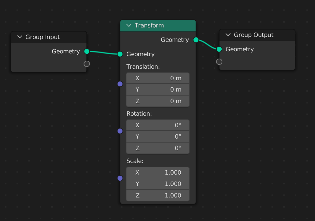
Now we can adjust the translation, rotation and scale values to transform our object and see the result in the 3D viewport in real time.
The transform node operates on the object level. While the origin of the object doesn't move, we are still transforming the whole mesh as a single element using this node.
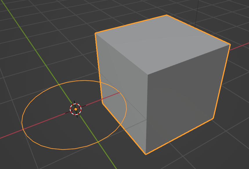
Another new feature that comes with geometry nodes is that we can now have an object contain other types of geometry that it couldn't before. For instance, we can add a curve primitive, such as a circle to our mesh object and both types of geometries will be contained inside the same object.
Try this.

Note that both the circle and the cube is located next to each other in the 3D viewport and they are contained in the same object even if the data they are made up of is different and wouldn't normally be part of the same object type.
Something to keep in mind here is that geometry nodes is a modifier. If we applied the modifier, the data that doesn't fit into the host object type, in this case a mesh object, any other kind of geometry gets deleted.
So we cannot have both curve data and mesh data in the same object outside of geometry nodes.
Also, note the elongated input socket on the join geometry node. This is a new type of socket that takes any number of inputs and joins them together to output a combined output. in this case, a combined geometry output.
We can add any kind of mesh or curve primitive into an existing geometry nodes tree from the add menu and join them using the join geometry node.
In geometry nodes we have these teal colored inputs and outputs that control the flow of data. But within a teal geometry socket we have five different kinds of data and different nodes take different inputs and sends different outputs even if the color is the same.
We can view it as a hierarchy where the geometry is the container and these five subcomponents make up the geometry.
Each of these are different kinds of geometry.
By using the separate component node, we can separate each of these geometry types from a combined geometry and use only that component as input for another node.
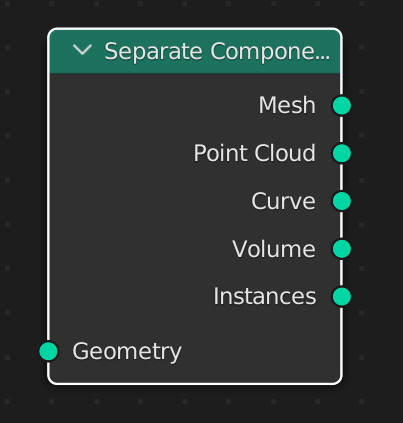
You may have noticed that different nodes have a different label on their teal input and output sockets. Even the separate components node has the same colored output sockets but each of them output different kinds of data.
Another example, the instance on points node that we use to scatter objects on another object takes two green socket inputs. A point input and an instance input. If we input another kind of data with a teal socket, such as mesh data or curve data, Blender sometimes interpret between the two types and sometimes throws an error.
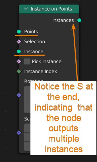
Just make sure that you input the correct type of data even if the sockets have the same color.
Another example are vector data, a rotation value is different from a position value, yet they are both vector data and have a purple input and output socket.
An abstract way of explaining fields is to say that a field is a function. While this is true, it can be hard to understand what this means in practice. You may also have heard that a field does not contain any data. This is also true. Let's explore fields in geometry a bit further to explain what is really going on.
Imagine that you have a spreadsheet filled with information about something. It could be anything, but for this example let's pretend that it is a spreadsheet of your budget. All your expenses and earnings.
This would be data stored on your hard drive. You could manipulate it, change it or display it in various ways. But it is only your budget. Now imagine that you needed to budget for a friend. You would need to setup a new spreadsheet, insert all the data according to your friends bank account and manage and store two separate spreadsheets.
That would be double the amount of work. Now image that you have to this for 100 friends and it would quickly become unmanageable.
Instead, let's say that the bank allowed a direct connection to your accounts and in your spreadsheet, you could now directly pull the data from your account in real time as transactions happen to your account. So every time there is an update at your bank, it would automatically get updated in your spreadsheet.
In fact, there would be no need to store any data in your spreadsheet anymore, you could just store a set of functions that run when you open the spreadsheet to pull the data in in the order that you want at that point in time.
You can now use this function for all your 100 friends accounts and there is no extra work.
This is kind of what a field is. It generates the data based on the context. Just replace each of your friend with geometry, and each of your accounts, expenses and earnings with data within that geometry. It can be the position of each vertex in the mesh or the normal direction of each face in a subset of the geometry for example.
A field is a collection of data that is generated based on the context.
In programming, this is called a higher order function. It is a function that can be passed as a variable, but a function does not contain data, instead it is ran in the context of the function it is passed into and therefore the data that it generates is used as the input.
But if you are not a programmer or understand what this means, just ignore it and stick to the spreadsheet analogy.
Let's take a look at what it looks like inside the node editor.
Now when we know the idea behind fields. Let's look at them in practice. To distinguish a field from regular data being passed around we need to look at the connection between nodes and the input and output sockets.
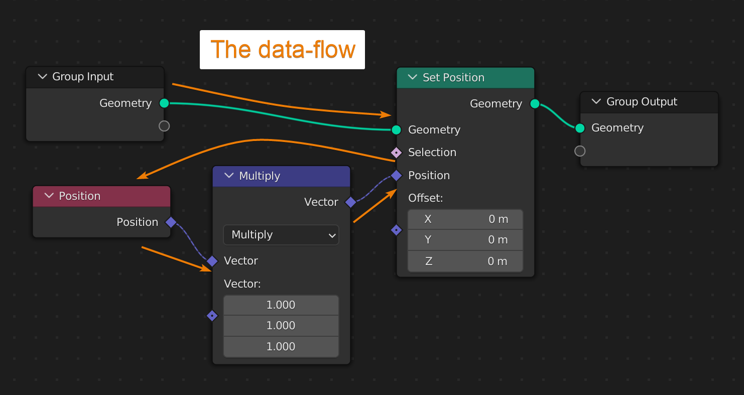
In this image we see a basic setup where we change the position using the set position node. By changing the offset values we can move our input geometry around in the X, Y and Z coordinates. With the vector math node set to multiply we can use these sets of values to scale our object.
To understand fields we have to look at how execution flows in the graph. The execution flow follows the teal geometry connections and at every teal node, Blender stops, look at the other inputs and evaluate each of them.
In this example our original geometry comes from the group input node and is passed to the set position node. At this point Blender uses the default value for the selection input and the offset input get whatever value we manually input. In this case it is currently set to 0 for each axis.
For the position node however, Blender backtracks and start at the position node, then goes through the multiply node and end back at the position input of the set position node. Here it uses the result of the position and multiply node as its value.
In this case the position node outputs a field. This means that the data it outputs is based on the context and the context is the geometry that the set position node gets as input from the group input node.
We can say that the position node contains the position of each element of the geometry that is its context. In case of a mesh object, this is the position of each vertex.
In programming terms the set position node would look something like this.
set_position_node(Selection=All, Position=Multiply(Position(), Vector(0,0,0)), offset(0,0,0))
To get the position, the position function needs to be evaluated first, then the multiply vector function.
In the Blender manual, there is a differentiation between data-flow nodes and field nodes that pass data. In this case the group input passing data to the set position and then passing data to the output node is the data-flow.
The position and vector math node are field nodes or data that needs to be evaluated before the data-flow can continue.
In this case the position has no meaning on its own. It only has meaning when it is used in the context of some kind of geometry. This doesn't necessarily have to be a mesh object. It could be a point cloud, a curve, volume or instance. Depending on the kind of geometry the position mean different things.
Most data-flow nodes are nodes that pass geometry as output. An example of a node that isn't a data-flow node but that may seem like on is the Geometry proximity node that takes geometry as input, but it doesn't pass geometry as output and therefore it is not a data-flow node. But the set position node is a data-flow node since it passes the geometry to the next step in the node graph.
External content: Geometry nodes: Fields, Blender manual
By now we have a good understanding of the flow of data. You should also have noticed the different kinds of sockets involved. There are three kinds,
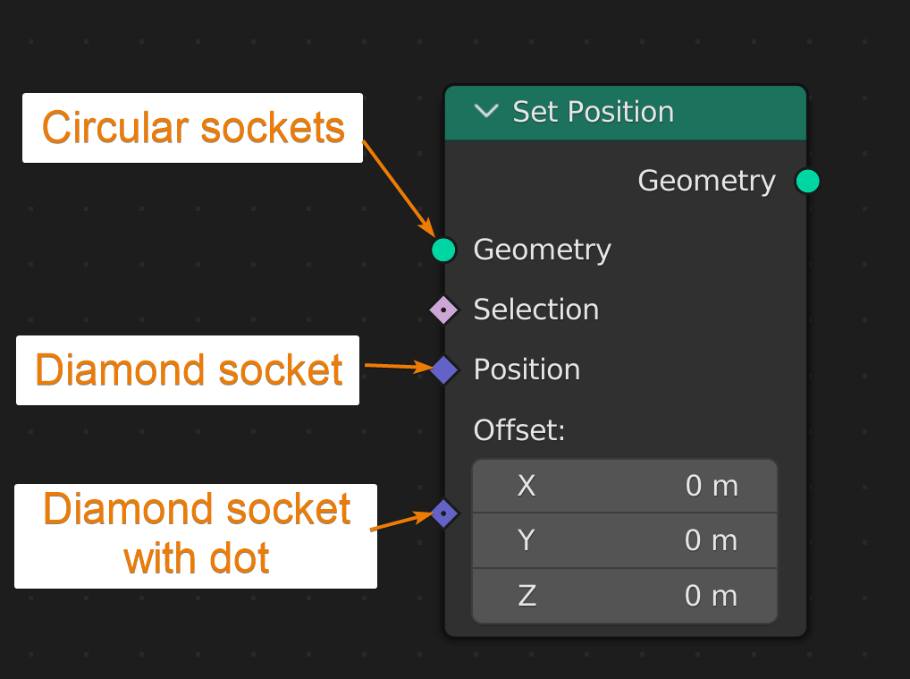
The diamond sockets indicate that it is a field input. Field inputs can also take general data as input that otherwise go through circular sockets. If a socket can take field input but is currently not taking a field as an input, it is indicated by the diamond socket with a dot in the middle.
So in the set position node here, we have circular, data input for the geometry. geometry is always data. After that we have the selection input that can be used to select a portion of our geometry that the set position affects. It can take a field as input but is currently a fixed value input. In this case the default value is everything. So it affects the whole geometry.
The position input takes the position of each element as input. In the case of a mesh geometry, this would be the position of each vertex of the mesh plugged into the geometry input. This is the same as using the position node and directly input it into this slot. In other words, it is a field that is currently using field data.
The last slot is the offset that is currently taking data as input. The data can be set on the node itself. But we could input a field here.
The color indicate what kind of data the socket output or input. But we also have to be careful to also look at the wording on the node to know exactly what data we are dealing with. But let's start with the color. Here is a list of possible socket colors.
| Socket color | Data type | Can be a field |
|---|---|---|
| Teal | Geometry | No |
| Gray | Float value | Yes |
| Purple | Vector values | Yes |
| Yellow | Color value | No |
| Dark green | Integer value | Yes |
| Red | Material | No |
| Pink | Boolean | Yes |
| Light blue | String | No |
It is easy to think that the same data types are always compatible, but this is not the case. The data type just refers to the storage format of the data. But data that is stored similarly can have very different use cases.
For instance, a geometry output could contain one or more of these kinds of data like we touched on earlier.
But inputting geometry data that is made up of curve data is not the same as inputting geometry that is made up of mesh data for example. Therefore we need to know what data we are passing around.
Similarly vector data is not always position data, it could contain a rotation or a scale.
We have the opposite situation between color data and vector data. These two kinds of input is similar and sometimes we can use them in place of each other. For instance, normal maps is an example where vector data is stored as color.
Blender will also automatically try to convert between data types. So for vector and color, The X, Y and Z values will be mapped to the R, G and B colors in that order.
The bottom line is that we need to know what data we are passing around and how it relates to other types of data when we want to go from one type to another.
Let's look at how we can bring in external data to work with. A couple of common kinds of data to bring in is UV maps or weight painted vertex groups.
To bring in these kinds of data that is part of our geometry we use the group input node to add a socket. In the modifier tab we can then add a variable as input.
Let's look at vertex groups as the example.
Related content: How to use vertex groups in Blender
Select the group input node, if you removed it, just press Shift+A go to Group->Group input to add one back in.
We can have multiple group input nodes. It can help to keep the node graph cleaner and easier to read.
First we need to create a socket for the kind of data we want to bring in from an external source. A vertex group happens to be float value data since it keeps a value between zero and one for each vertex in your mesh.
We can either take an existing gray colored input socket of any node and plug it backwards into the output of the group node to create the output we need.
We can also select the group node, press N to bring up the right-side toolbar, and go to the group tab. Here we have an input section and an output section. Click the plus icon in the input section to add an input slot.
We can then specify the type, maximum and minimum value, tooltip etc.
For vertex groups, we can setup a float, give it a name and set the min to zero and max to one.
Then navigate to the modifier tab in the properties panel and our inputs will be listed on the geometry nodes modifier.
We can input a value that corresponds to the setting we just configured, or we can click the icon to the left of the input that looks something like a flag or a cross in a box. Next select from the list or search for the name of your vertex group.
If the vertex group isn't created, we can type a name, go to the object data properties, that is the green triangle icon, and create a vertex group in the vertex group section.
The name we give our group will be the name we need to input in the geometry nodes modifier input.
We can now access this external vertex paint data inside our geometry nodes graph.
In case of geometry nodes, attributes are data that belong to a certain geometry. For instance, the position of all vertices in a mesh or all the angles of all the faces in a mesh.
It could also be all the control points along a curve, a vertex group or uv map data to give a few examples. It is data that belongs to a specific object.
An example of something that is not an attribute, is a color or the output from a procedural texture such as a noise texture. These kinds of data do not belong to a specific object.
We pass attributes through fields.
We have two kinds of attributes in geometry nodes, named attributes and anonymous attributes.
A named attribute is something that is known beforehand. For instance, we know that the position attribute contains position data, or the normal attribute contain normal data. Or I should say, the normal and position fields point to the normal and position attributes of the given geometry in the node tree as discussed in the fields section above.
Related content: What are normals and how do they work in Blender?
But sometimes data needs to be anonymous, or it needs to become anonymous to be used at the right time in the node tree. This is where the capture attribute node come into play. Let's look at what I mean.
The capture attribute node allows us to take an attribute and either store it directly at a certain point in time in the node graph or to evaluate something that requires data from a particular time in the node tree. For instance, before we convert the data needed to another kind of data. We can then use this as an anonymous attribute later in the node tree.
We will demonstrate this with a simple example. Here is the node tree that I have setup.

This geometry node tree creates this result.
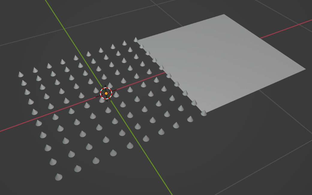
Not much to look at but let me explain what is happening.
We start by adding a grid that is 10 by 10 vertices. We then capture the position of each point in this grid using the position node together with a capture attribute node set to the data type of vector and the attribute of position.
This essentially captures the position of each vertex in the grid.
We then change the position of the grid by moving it 1 full unit in the X direction with the set position node.
Next, we use an instance on points node and a cone to create a cone at every vertex of our object. To be able to see what is happening a bit better I used the scale values on the instance on points node to scale the cone down considerably.
Now this is where the magic happens. Since we stored the previous location of our grid before we changed it, we can now set the position of our cones to be the position of the original vertex locations before we changed it with the first set position node.
Related content: How to scatter objects with geometry nodes in Blender
This is a very simple example that by itself isn't very useful. But what this means is that we can capture any attribute at any point in time and throw it as input later when some data has changed.
The attribute created by the capture attribute node here is what we call an anonymous attribute. It may sound complex, but it is really just a node output.
We covered not only the introduction and basics of geometry nodes but core fundamentals, such as the flow of operations, what are fields and how to get data into geometry nodes from external sources. This is the fundamentals to later build on when you start to come up with your own geometry nodes project.
Just remember that everything doesn't suddenly have to be made with geometry nodes. Instead, think about what kind of problem you are facing and think about the kind of tool and solution that would be of best help to solve that particular problem. While geometry nodes will be the answer in many cases it is easy to think that it is the solution to end all other tools. Instead, let it complement what you already know.
Thanks for your time
